Abstract

Contents

This page follows the manuscript closely. It is written as mathematical exposition rather than as a summary page.

Article type: research

1 Introduction

The classic Fibonacci Tiling begins with two squares with side lengths \(1\) and uses the recurrence \(F_n=F_{n-1}+F_{n-2}\) to continuously add squares with side-lengths of the Fibonacci numbers sequentially. These squares are added in a pattern of up, left, down, right and repeats to create an expanding rectangle. In each of these squares, a quarter circle is drawn, creating the familiar Fibonacci Spiral. We study a sequential randomization of this construction. The axis on which we add the subsequent square alternates deterministically, but a fair coin decides which side the next square is added onto the current rectangle. The first goal of this paper is to determine the expected covering time of a fixed lattice point on the plane, i.e., the first added square of the rectangle to cover a specific point. Our second goal is to extend the Fibonacci spiral to our randomized construction.

The main probabilistic simplification is to track the rectangle’s boundary instead of the individual squares. Each time an axis is updated, one of its two boundary faces moves outward by a deterministic amount. The distance traveled by a particular face is therefore a sum of fixed weights selected by independent coin flips. In the plane, these weights are the even- or odd-indexed Fibonacci numbers. Moreover, the two coordinate-covering times depend on disjoint sets of coin flips and are independent. The point is covered when both coordinate conditions hold, so its covering time is the maximum of these two times.

The same approach extends to \(d\)-dimensional blocks whose attachment axes cycle through the coordinate directions. The dimension of the growing cuboid is governed by the recurrence \(F_n^{(d)} = F_{n-1}^{(d)} + F_{n-d}^{(d)}\). We look at the subsequences modulo \(d\) and obtain super-increasing sequences which allow us to proceed in a similar fashion as the two-dimensional case. This observation turns a covering condition into a threshold in a binary ordering of subsets, providing exact counts of the coin-flip outcomes that cover a given coordinate.

Corollary 23 gives \[\label{eq:intro-covering-asymptotics} \mathbb{E}[T(a)]\ =\ \frac{\log \delta_\infty(a)}{\log \rho_d} +O_d(1), \qquad \operatorname{Var}(T(a))\ =\ O_d(1)\] as \(\delta_\infty(a)\to\infty\), where \(T(a)\) is the covering time of the lattice point \(a\), \[\label{eq:intro-target-distances} \delta_r(a)\ =\ \max\{a_r-1,-a_r,0\}, \qquad \delta_\infty(a)\ =\ \max_{0\leq r<d}\delta_r(a),\] and \(\rho_d>1\) is the positive root of \(x^d-x^{d-1}-1=0\). Since the initial block is \([0,1]^d\), one also has \(\delta_\infty(a)=\|a\|_\infty+O(1)\) as the target recedes to infinity.

For the spiral construction, random placements are incompatible with the quarter-circles from meeting with the required endpoints and tangents. We address this square by square, assigning exactly one curve segment to each square. Standard configurations retain their quarter-circles, while nonstandard configurations use a quintic connector followed by a circular arc. The construction requires the placement of the next square, so it uses one-step lookahead. It produces a curve admitting a continuously differentiable parametrization and recovers the standard Fibonacci spiral. Containment and self-intersection remain separate geometric questions.

The paper is organized as follows. Section 2 defines the planar and higher-dimensional tilings and develops the d-dimensional recurrence. Section 3 establishes the super-increasing and canonical-ordering results for coordinate subset sums. Section 4 derives the exact \(d\)-dimensional covering formulas. Section 5 proves the limiting results, including bounded fluctuations and the dependence of the growth scale on \(d\). Section 6 constructs the random spiral and records the remaining geometric questions. Notation is collected in Appendix 8

[top]

2 Random Tiling Construction

2.1 The planar construction

Let \(\{F_n\}_{n\geq0}\) denote the Fibonacci sequence with \[\label{eq:fibonacci-sequence} F_0\ =\ F_1\ =\ 1, \qquad F_n\ =\ F_{n-1}+F_{n-2} \quad(n\ \geq\ 2).\] Begin with the fixed unit square \([0,1]^2\). We count only subsequent square appendages as moves.

Let \((c_n)_{n\geq 1}\) be independent Bernoulli random variables satisfying \[\label{eq:fair-placement-coins} \mathbb P(c_n\ =\ 0)\ =\ \mathbb P(c_n\ =\ 1)\ =\ \frac12.\] At move \(n\), append an \(F_n\times F_n\) square to the current rectangle. When \(n\) is odd, attach the square to the right if \(c_n=0\) and to the left if \(c_n=1\). When \(n\) is even, attach it to the top if \(c_n=0\) and to the bottom if \(c_n=1\). Thus odd moves expand the construction horizontally and even moves expand it vertically. We use the convention \(0=\) right/up and \(1=\) left/down throughout.

The random choices determine the position of the growing rectangle but not its side lengths. After \(n\) moves, its side lengths are \[\label{eq:planar-side-lengths} F_n\quad\text{and}\quad F_{n+1},\] up to permutation according to the parity of \(n\). Indeed, the initial square has dimensions \(F_0\times F_1\), and at each move the newly attached square has side length equal to the longer side of the current rectangle. The shorter side is therefore replaced by the sum of the two preceding side lengths.

Figures 1 and 2 illustrate two realizations. With the convention above, that \(0=\) right/up and \(1=\) left/down the corresponding words are \([0,0,0,0]\) and \([0,0,1,0,0]\), respectively. A word records all directional choices, but extracting the absolute position of the rectangle from that word leads to a weighted subset-sum problem developed in Section 3.

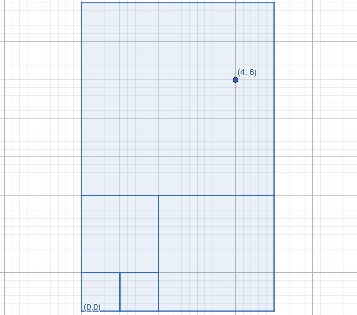
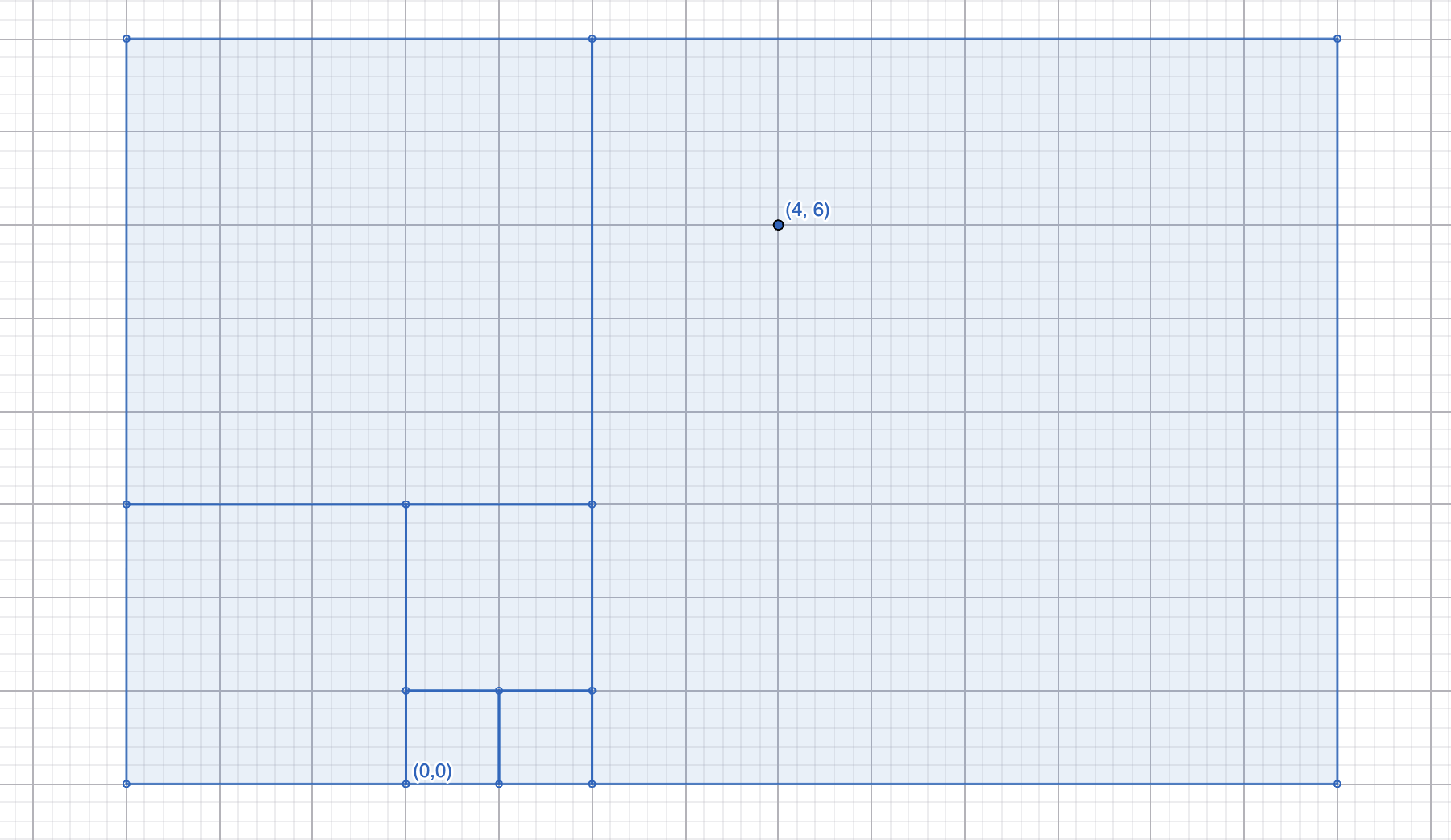
The construction gives rise to two principal questions. First, for a lattice point \((a,b)\in{\mathbb Z}^2\), how many moves are required, on average, before the growing rectangle covers \((a,b)\)? Second, how can the Fibonacci spiral from the standard deterministic tiling be extended to this random setting?

2.2 The higher-dimensional construction

The planar process has a natural cyclic extension to dimension \(d\geq 2\). Begin with the unit hypercube \([0,1]^d\). At move \(k\geq1\), update coordinate \(r\equiv k-1\pmod d\), with \(0\leq r<d\). Use the independent fair placement bits \((c_k)_{k\geq1}\), where \(0\) selects the positive face and \(1\) selects the negative face. At successive moves, choose the coordinate axes in a fixed cyclic order. Along the selected axis, a fair coin determines whether the new block is attached to the positive or negative face. The new block spans the entire exposed \((d-1)\)-dimensional face, and its thickness is equal to the most recently created side length. Equivalently, at each move the side length that has gone one complete coordinate cycle without being updated is replaced by its sum with the most recently created side length.

This geometric rule motivates the following recurrence. The sequence is the specialization \(u(n;d-1,1)\) of Harris and Styles [3]; its recurrence and spectral properties are classical.

For \(d=2\), the exposed face has length \(F_k^{(2)}\) and the appended block has the same thickness, so it is an \(F_k^{(2)}\times F_k^{(2)}\) square. Hence the construction reduces exactly to the planar Fibonacci tiling. For \(d=3\), the recurrence \[\label{eq:narayana-recurrence} F_n^{(3)}\ =\ F_{n-1}^{(3)}+F_{n-3}^{(3)}\] is the Narayana recurrence [5], and the appended objects are generally rectangular cuboids rather than cubes.

We next record the growth properties needed in the covering-time analysis. Many properties of this sequence are intuitively borrowed from the Fibonacci sequence itself.

Proposition 4 is the structural input for the covering-time argument: it orders subset sums by their largest differing weight.

We define the dominant root of the recurrence, which provides information about the growth rate of the sequence.

2.3 Covering times

Let \(\mathcal{R}_n^{(d)}\) denote the random bounding hyperrectangle after \(n\) completed moves. For a lattice point \(a=(a_0,\ldots,a_{d-1})\in{\mathbb Z}^d\), define \[\label{eq:target-distances-active-set} \delta_r(a)\ =\ \max\{a_r-1,-a_r,0\}, \qquad I(a)\ =\ \{r:\delta_r(a)\ >\ 0\}.\] Thus \(\delta_r(a)\) is the distance from the appropriate face of \([0,1]^d\) to the target in coordinate \(r\), and \(I(a)\) is the set of coordinates not already covered initially. Define the covering time by \[\label{eq:covering-time-definition} T(a)\ =\ \inf\{n\ \geq\ 0:a\in\mathcal{R}_n^{(d)}\}.\] The first problem of the paper is to determine the distribution and moments of \(T(a)\), beginning with \[\label{eq:covering-time-objective} \mathbb{E}[T(a)].\] Although the side lengths of \(\mathcal{R}_n^{(d)}\) are deterministic, its position depends on the coin-flip word. Determining whether a given point has been covered is therefore equivalent to ordering certain weighted subset sums. The \(j\)^th update of coordinate \(r\) occurs at move \(r+1+jd\) and has thickness \[\label{eq:coordinate-weight-definition} w_{r,j}\ :=\ F_{d-1+r+jd}^{(d)}, \qquad j\ \geq\ 0.\] For each fixed \(r\), these weights form a tail of a residue-class subsequence, so Proposition 4 supplies the key structural fact for the analysis in the next section.

The second problem, the construction and analysis of a random Fibonacci spiral, uses the same sequence of appended blocks but tracks distinguished corners rather than the entire bounding hyperrectangle. We save its formal introduction for Section 6.

[top]

3 Weighted Subset Sums and Canonical Ordering

The side lengths of the random tiling are deterministic, but the position of the bounding hyperrectangle depends on the directions selected by the coin flips. Along each coordinate axis, the distance traveled toward a fixed target is therefore a weighted subset sum. We show that the terms associated with any one coordinate form a superincreasing sequence. It follows that their subset sums are ordered exactly as binary integers, which yields a canonical threshold word and an exact finite-time covering probability.

Throughout this section, let \(\left\{F_n^{(d)}\right\}_{n\geq0}\) be the order-\(d\) Fibonacci sequence defined by \[\label{eq:recurrence-recall} F_0^{(d)}\ =\ \cdots\ =\ F_{d-1}^{(d)}\ =\ 1, \qquad F_n^{(d)}\ =\ F_{n-1}^{(d)}+F_{n-d}^{(d)} \text{ for } n\ \geq\ d.\]

3.1 Coordinate subsequences and random subsets

Fix \(r\in\{0,1,\ldots,d-1\}\). The \(j\)^th update of coordinate \(r\), indexed from \(j=0\), occurs at move \(r+1+jd\) and moves the selected face by \[\label{eq:coordinate-weight-recall} w_{r,j}\ :=\ F_{d-1+r+jd}^{(d)}.\] For \(m\geq0\), define the first \(m\) coordinate weights and their cumulative sum by \[\label{eq:coordinate-weight-set-sum} \mathcal W_{r,m}\ :=\ \{w_{r,0},\ldots,w_{r,m-1}\}, \qquad W_{r,m}\ :=\ \sum_{j=0}^{m-1}w_{r,j},\] with \(\mathcal W_{r,0}=\varnothing\) and \(W_{r,0}=0\). Proposition 4 gives \[\label{eq:coordinate-superincreasing} w_{r,k}\ >\ W_{r,k} \qquad(k\ \geq\ 1),\] so every coordinate-weight sequence is superincreasing.

Let \(n\geq0\) denote the number of completed moves. The number of updates of coordinate \(r\) among those \(n\) moves is \[\label{eq:update-count} u_r(n)\ :=\ \#\{0\ \leq\ i\ <\ n:i\equiv r\pmod d\}\ =\ \begin{cases} 0,&n\ \leq\ r,\\[1mm] 1+\left\lfloor\dfrac{n-1-r}{d}\right\rfloor,&n\ \geq\ r+1. \end{cases}\]

Let \(a=(a_0,\ldots,a_{d-1})\in{\mathbb Z}^d\) be the target point and fix an active coordinate \(r\in I(a)\). Write \(\delta_r=\delta_r(a)>0\). Let \(\xi_{r,j}=1\) when the \(j\)th update of coordinate \(r\) is directed toward the target and \(\xi_{r,j}=0\) otherwise. Depending on which side of the initial cube contains the target, \(\xi_{r,j}\) is either \(c_{r+1+jd}\) or \(1-c_{r+1+jd}\) from the global placement sequence. Thus the coordinate variables are independent Bernoulli variables with parameter \(1/2\). After \(n\) completed moves, define \[\label{eq:random-coordinate-subset} E_{r,n}\ :=\ \{w_{r,j}:0\ \leq\ j\ <\ u_r(n),\ \xi_{r,j}\ =\ 1\} \subseteq\mathcal W_{r,u_r(n)}.\] Then the target has been covered in coordinate \(r\) after \(n\) moves exactly when \[\label{eq:coordinate-covering-event} \sum_{w\in E_{r,n}}w\ \geq\ \delta_r.\]

For \(E\subseteq\mathcal W_{r,m}\), define \[\label{eq:subset-membership-word} x(E)\ =\ (x_{m-1},\ldots,x_0)\in\{0,1\}^m, \qquad x_j\ =\ \begin{cases} 1,&w_{r,j}\in E,\\ 0,&w_{r,j}\notin E. \end{cases}\] Its weighted value is \[\label{eq:weighted-word-value} V_r(x)\ :=\ \sum_{j=0}^{m-1}x_jw_{r,j}\ =\ \sum_{w\in E}w.\]

3.2 Binary order and the canonical threshold

For \(x=(x_{m-1},\ldots,x_0)\in\{0,1\}^m\), define \[\label{eq:binary-rank-definition} \operatorname{rank}_2(x)\ :=\ \sum_{j=0}^{m-1}x_j2^j.\] For distinct words \(x,y\), let \(k(x,y)=\max\{j:x_j\neq y_j\}\). We write \(x<_{\mathrm{MSB}}y\) when \(x_{k(x,y)}<y_{k(x,y)}\).

The superincreasing property, standard in subset-sum problems [4], means that the largest weight on which two subsets differ outweighs every possible contribution from smaller weights. Thus this single digit determines the order of their weighted sums.

For the positive coordinate distance \(\delta_r\), define \[\label{eq:coordinate-threshold} m_r\ :=\ \min\{m\ \geq\ 1:W_{r,m}\ \geq\ \delta_r\}.\] This is the first coordinate-update count at which coverage is possible.

Minimality of \(m_r\) gives \(W_{r,m_r-1}<\delta_r\), so the leading digit of \(x_r^\star\) is \(1\). Therefore \[\label{eq:threshold-rank-bounds} 2^{m_r-1}\ \leq\ R_r\ <\ 2^{m_r}, \qquad \frac12\ \leq\ \kappa_r\ <\ 1.\]

3.3 The exact coordinate covering law

Fix \(r\in I(a)\), and define \[\label{eq:coordinate-time-definitions} \tau_r\ :=\ \inf\left\{m\ \geq\ 0: \sum_{j=0}^{m-1}\xi_{r,j}w_{r,j}\ \geq\ \delta_r\right\}, \qquad b_r\ :=\ r+1+d(m_r-1).\] Here \(\tau_r\) counts updates of coordinate \(r\), whereas \(T_r\) denotes the first global move at which that coordinate is covered.

The key observation is that every weight appearing after the first feasible update count already exceeds the target distance. Continued failure therefore requires every newly exposed bit to be zero.

In particular, if \(u_r(n)\) is the number of coordinate-\(r\) updates among the first \(n\) moves, then \[\label{eq:coordinate-survival} \mathbb P(T_r\ >\ n)\ =\ \begin{cases} 1,&u_r(n)\ <\ m_r,\\ R_r2^{-u_r(n)},&u_r(n)\ \geq\ m_r. \end{cases}\]

[top]

4 Covering Time in \(d\) Dimensions

We combine the coordinate subset-sum formulas to obtain the covering-time distribution for a target point \[\label{eq:target-vector} a\ =\ (a_0,a_1,\ldots,a_{d-1})\in{\mathbb Z}^d.\]

Recall that \[\label{eq:active-set-recall} \delta_r\ =\ \delta_r(a)\ =\ \max\{a_r-1,-a_r,0\}, \qquad I\ =\ I(a)\ =\ \{r:\delta_r\ >\ 0\}.\] Coordinates outside \(I\) are already covered by the initial hypercube; for them set \(T_r=0\). We assume below that \(I\neq\varnothing\); if \(I=\varnothing\), then \(T(a)=0\).

For \(r\in I\), the update count, feasibility threshold, and coordinate survival law are given by [eq:update-count], [eq:coordinate-threshold], and [eq:coordinate-survival], respectively.

4.1 Coordinate independence and the exact distribution

Let \(c_k\) be the placement bit used at move \(k\geq1\). Coordinate \(r\) depends only on the flips \[\label{eq:coordinate-coin-subsequence} c_{r+1},\ c_{r+1+d},\ c_{r+1+2d},\ \ldots.\]

4.2 Cycle decomposition of the geometric tail

Let \[\label{eq:maximal-threshold} m_*\ :=\ \max_{r\in I}m_r.\] Write the number of completed moves as \(n=dk+s\), where \(0\leq s<d\). Then \[\label{eq:cycle-update-count} u_r(dk+s)\ =\ k+\mathbf{1}_{\{r<s\}}.\] In particular, if \(k\geq m_*\), every active coordinate is in its geometric regime and \[\label{eq:cycle-coordinate-tail} \overline F_r(dk+s)\ =\ \frac{R_r}{2^{k+\mathbf{1}_{\{r<s\}}}}.\]

For a nonempty subset \(J\subseteq I\), define \[\label{eq:subset-phase-data} R_J\ :=\ \prod_{r\in J}R_r, \qquad \eta_s(J)\ :=\ \#\{r\in J:r\ <\ s\}.\]

To shorten the moment formulas, define the phase sums \[\label{eq:phase-sums} H_J\ =\ \sum_{s=0}^{d-1}2^{-\eta_s(J)} \quad\text{ and }\quad K_J\ =\ \sum_{s=0}^{d-1}(2s+1)2^{-\eta_s(J)}.\] Both depend only on the positions of the coordinates in \(J\) within the cyclic update order.

4.3 Moment Formulas

For a nonnegative integer-valued random variable, \[\label{eq:expectation-tail-sum} \mathbb{E}[T]\ =\ \sum_{n=0}^{\infty}\mathbb{P}(T\ >\ n).\] We split this sum immediately before the first complete geometric cycle as \[\label{eq:expectation-split} \mathbb{E}[T]\ =\ E_{\mathrm{fin}}+E_{\mathrm{tail}},\] where \[\label{eq:expectation-finite-part} E_{\mathrm{fin}}\ =\ \sum_{n=0}^{dm_*-1}\mathbb{P}(T\ >\ n).\]

Although the original tail is an infinite series, the theorem expresses it as a sum over the \(2^{|I|}-1\) nonempty active-coordinate subsets. Thus, for fixed \(d\), the only unsummed part is the finite transient range \(0\leq n<dm_*\).

The second tail-sum identity is \[\label{eq:second-moment-tail-sum} \mathbb{E}[T^2]\ =\ \sum_{n=0}^{\infty}(2n+1)\mathbb{P}(T\ >\ n).\] Define \[\label{eq:second-moment-finite-part} M_{2,\mathrm{fin}}\ =\ \sum_{n=0}^{dm_*-1}(2n+1) \left[ 1-\prod_{r\in I}\bigl(1-\overline F_r(n)\bigr) \right].\]

[top]

5 Limiting Behavior

Theorems 17, 19, and 20 of Section 4 determine the covering-time distribution for every fixed target. We use them to describe the behavior of the covering time as the target moves away from the initial hypercube. We show that the expected covering time grows logarithmically, the excess beyond its deterministic threshold has a uniformly exponential tail, and all centered moments remain bounded when the dimension is fixed.

Throughout this section, \(d\geq2\) is fixed and \(I(a)\neq\varnothing\). For \(a\in{\mathbb Z}^d\), recall \[\label{eq:limiting-target-distances} \delta_r(a)\ =\ \max\{a_r-1,-a_r,0\}, \qquad I(a)\ =\ \{r:\delta_r(a)\ >\ 0\},\] and write \[\label{eq:limiting-distance} \delta_\infty(a)\ :=\ \max_{0\leq r<d}\delta_r(a).\] When the target is fixed, we abbreviate \(\delta_r=\delta_r(a)\) and \(I=I(a)\). For \(r\in I(a)\), let \(b_r=r+1+d(m_r-1)\) be the earliest move at which coordinate \(r\) can be covered, and let \[\label{eq:earliest-full-covering} B(a)\ :=\ \max_{r\in I(a)}b_r\] be the earliest move at which all active coordinates can be covered.

5.1 Deterministic location

For each active coordinate, minimality of \(m_r\) gives \[\label{eq:threshold-bracketing} W_{r,m_r-1}\ <\ \delta_r\ \leq\ W_{r,m_r}.\]

5.2 Uniform fluctuations and their consequences

Assume \(I(a)\neq\varnothing\). By Theorem 13, \(T_r=b_r+dG_r\) and \(\mathbb P(G_r>k)=\kappa_r2^{-k}\). Set \(G_{\max}:=\max_{r\in I(a)}G_r\). Since \(T=\max_{r\in I(a)}T_r\) and \(B(a)=\max_{r\in I(a)}b_r\), \[\label{eq:limiting-delay-comparison} 0\ \leq\ T-B(a)\ =\ \max_{r\in I(a)}\{b_r-B(a)+dG_r\}\ \leq\ dG_{\max}.\] Thus the fluctuations are controlled by at most \(d\) coordinate delays, each having a geometric tail independent of the scale of the target.

5.3 The centered covering-time law

Theorem 22 implies that \[\label{eq:tight-centered-family} \{T(a)-B(a):a\in\mathbb Z^d,\ I(a)\ \neq\ \varnothing\}\] is tight for fixed \(d\): its members are nonnegative and their tails are uniformly bounded by \(d2^{-k}\) at \(dk\).

The independent coordinate delays also give the exact identity \[\label{eq:maximum-delay-exact-tail} \mathbb P(G_{\max}\ >\ k)\ =\ 1-\prod_{r\in I(a)}(1-\kappa_r2^{-k}).\] Indeed, the coordinate delays depend on disjoint sets of independent placement coins. This identity is a law for \(G_{\max}\), not generally for \((T-B(a))/d\), because \[\label{eq:centered-covering-identity} T-B(a)\ =\ \max_{r\in I(a)}\{b_r-B(a)+dG_r\}.\] Consequently, the centered law depends on the active-coordinate set, the ranks \(\kappa_r\), and the offsets \(b_r-B(a)\). Tightness guarantees weakly convergent subsequences, but does not by itself identify a universal centered limiting law.

5.4 The planar case

When \(d=2\), coordinate \(0\) uses the odd-indexed Fibonacci numbers \(F_{1+2j}\), coordinate \(1\) uses the positive even-indexed Fibonacci numbers \(F_{2+2j}\), and \[\label{eq:planar-dominant-root} \rho_2\ =\ \varphi\ =\ \frac{1+\sqrt5}{2}.\]

5.5 Dependence on the dimension

We finally allow \(d\to\infty\) to examine the coefficient of \(\log \delta_\infty(a)\) in the deterministic scale. Let \(\operatorname{W}_0\) denote the principal real branch of the Lambert function [1], defined by \(\operatorname{W}_0(x)e^{\operatorname{W}_0(x)}=x\) for \(x>0\).

This comparison concerns the deterministic growth scale only. The bounds denoted by \(O_d\) may depend on \(d\), so these results do not by themselves establish a joint limit in which both dimension and target distance grow.

[top]

6 Random Fibonacci Spirals

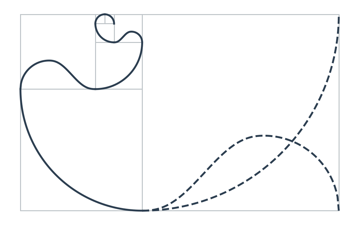
The standard Fibonacci spiral is obtained by inscribing a quarter-circle in each square of the standard Fibonacci tiling. Consecutive arcs meet at square corners with a common tangent, producing a continuously differentiable curve. In the random tiling, however, the placement of the next square may require the curve to leave the current square through a different corner. A fixed choice of quarter-circles need not then have the correct exit point or tangent.

We construct the random spiral one square at a time. Each square is assigned exactly one curve segment. The initial square has index \(0\), and the square appended at move \(n\geq1\) has side length \(F_n\). The segment in the square of side length \(F_n\) is determined after the placement of the square of side length \(F_{n+1}\) is known. Thus the construction uses one-step lookahead and is not a causal process.

The local quintic connector used in Theorem 28 was proposed by László Szalay in discussions following the conference problem session.

Let \(\mathcal Q_n\) denote the square of side length \(F_n\), and let \[\label{eq:spiral-placement-word} \omega\ =\ (\omega_1,\omega_2,\ldots)\in\{0,1\}^{\mathbb N}\] be the realized placement word, with \(\omega_n=c_n\), determining the placements of the squares. The curve segment assigned to \(\mathcal Q_n\) is denoted by \(\gamma_n\). We take \(\gamma_0\) to be the usual quarter-circle in the initial unit square.

For \(n\geq1\), the preceding segment determines an entrance corner of \(\mathcal Q_n\) and an incoming tangent direction. Once \(\mathcal Q_{n+1}\) has been placed, its location determines the required exit corner of \(\mathcal Q_n\) and the outgoing tangent direction. All local configurations are considered up to rotations and reflections.

We call the data in \(\mathcal Q_n\) standard if the usual quarter-circle of radius \(F_n\) joins the prescribed entrance and exit corners with the required tangents. Otherwise, we call the data nonstandard.

For \(n\geq1\), the square \(\mathcal Q_n\) is assigned its curve segment as follows.

1. If the data in \(\mathcal Q_n\) are standard, then \(\gamma_n\) is the usual quarter-circle of radius \(F_n\).

2. If the data in \(\mathcal Q_n\) are nonstandard, then \(\gamma_n\) is the composite of a quintic connector and an outgoing circular arc, as defined in [eq:nonstandard-segment].

In either case, the endpoint and terminal tangent of \(\gamma_n\) are used as the entrance data for \(\gamma_{n+1}\). Therefore the segment in \(\mathcal Q_n\) is defined only once: it is determined by the entrance data inherited from \(\mathcal Q_{n-1}\) and the exit data determined by the placement of \(\mathcal Q_{n+1}\).

Figure 3 illustrates the role of the next placement.

6.1 The local nonstandard segment

For the reference nonstandard configuration in a square \(\mathcal Q_n\), where \(n\geq1\), set \[\label{eq:connector-scales} A_n\ :=\ F_{n-1},\qquad B_n\ :=\ F_n,\qquad h_n\ :=\ \theta B_n,\qquad \varrho_n\ :=\ (1-\theta)B_n, \quad 0\ <\ \theta\ <\ 1.\] Take the entrance point to be the origin with the incoming tangent directed along the positive horizontal axis. The reference incoming arc and the outgoing arc are \[\label{eq:reference-circular-arcs} \begin{aligned} y_{n,-}(x)&\ =\ A_n-\sqrt{A_n^2-x^2}, &&-A_n\ \leq\ x\ \leq\ 0,\\ y_{n,+}(x)&\ =\ \sqrt{\varrho_n^2-(x-h_n)^2}, &&h_n\ \leq\ x\ \leq\ B_n. \end{aligned}\] The incoming arc is used only to prescribe endpoint data; it is not an additional piece inside \(\mathcal Q_n\). Let \(\sigma_5(t):=10t^3-15t^4+6t^5\).

The existence and uniqueness below are a two-node Hermite interpolation problem; see [2]. We retain the explicit polynomial for the geometric construction.

The reference nonstandard segment is \[\label{eq:nonstandard-segment} \begin{aligned} \gamma_n^{\mathrm{ref}}\ =\ {}&\{(x,P_n(x)):0\ \leq\ x\ \leq\ h_n\}\\ &\mathbin{\cup}\{(x,y_{n,+}(x)):h_n\ \leq\ x\ \leq\ B_n\}. \end{aligned}\] Whenever the prescribed local data are congruent to this configuration, transport this composite to the actual square by the corresponding rigid motion.

If the incoming segment is not the reference circle, matching its position and oriented tangent gives a geometric \(G^1\) join, but does not impose matching curvature. A \(C^1\) parametrization of the full concatenation requires compatible parameterizations of its pieces.

6.2 Definition and global regularity

6.3 Scaling and length

For \(n\geq1\), put \(\mu_n:=F_n/F_{n-1}\). The connector formula becomes \[\label{eq:normalized-connector-scaling} P_n(\theta F_n t)\ =\ F_ng_{\theta,\mu_n}(t),\] where \[\label{eq:normalized-connector-polynomial} g_{\theta,\mu}(t)\ =\ (1-\theta)\sigma_5(t) +\frac{\theta^2\mu}{2}t^2(1-t)^3 -\frac{\theta^2}{2(1-\theta)}t^3(1-t)^2.\] Thus the normalized connector shape depends only on \(\theta\) and \(\mu_n\). Define \[\label{eq:connector-length-integral} \Lambda(\theta,\mu)\ :=\ \int_0^1\sqrt{\theta^2+(g'_{\theta,\mu}(t))^2}\,dt.\] Let \(\mathcal L_n^{\mathrm{con}}(\theta)\) be the connector length in a nonstandard square, and let \(\ell_n=\operatorname{len}(\gamma_n)\).

6.4 Geometric questions

The square-by-square construction establishes that the random spiral is globally well-defined and \(C^1\), but several geometric properties remain open.

1. Choice of the splice parameter. Is there a canonical value of \(\theta\), such as \(1/2\) or \(\varphi^{-1}\)? Alternatively, should \(\theta\) minimize length, maximum curvature, or bending energy, where \(\mathcal K(s)\) denotes curvature at arclength \(s\), \[\label{eq:bending-energy} \int \mathcal K(s)^2\,ds?\]

2. Containment. For which values of \(\theta\) does every nonstandard segment remain inside its assigned square, or inside the union of the locally involved squares? The Hermite endpoint conditions alone do not rule out overshoot.

3. Curvature propagation. Instead of prescribing the entrance curvature \(1/F_{n-1}\), one could use the actual terminal curvature of \(\gamma_{n-1}\). Would this recursive choice produce \(C^2\) regularity across consecutive nonstandard squares while retaining acceptable containment and scaling properties?

4. Self-intersection and asymptotic shape. Is \(\Gamma_\theta(\omega)\) simple for every finite tiling word? If not, what is the probability of self-intersection under independent fair coin flips? How do its winding, radial growth, and rescaled shape depend on the tiling word?

5. Online constructions. Can one define a satisfactory random spiral without knowing the placement of the next square, or is one-step lookahead unavoidable under any natural corner and tangent rule?

6. Higher dimensions. Is there a natural curve, surface, or family of splines associated with the order-\(d\) tilings that reduces to the present construction in the plane?

[top]

7 Conclusion

We introduced a random growth model in which Fibonacci-sized blocks are attached along cyclically chosen coordinate axes while independent coin flips select the direction of each attachment. The dimensions of the growing block are deterministic, but its location is governed by weighted Bernoulli subset sums. Splitting the order-\(d\) Fibonacci sequence into its coordinate residue classes exposes the main structure of the model: each class is superincreasing. This gives unique subset sums, a most-significant-bit order, and canonical threshold words that convert geometric covering events into exact binary counts.

This representation leads to exact finite-time laws for the coordinate covering times and, by independence and inclusion–exclusion, for the full \(d\)-dimensional covering time. For fixed \(d\geq2\) and \(I(a)\neq\varnothing\), the dominant root \(\rho_d\) determines the macroscopic scale through \[\label{eq:conclusion-covering-scale} \mathbb{E}[T]\ =\ \log_{\rho_d}\delta_\infty(a)+O_d(1).\] At the same time, the centered fluctuations have exponential tails and moments bounded uniformly over the target. Thus the covering time becomes relatively concentrated even though bounded lattice and phase effects may prevent a single centered limiting distribution without passing to subsequences.

The random-spiral construction gives a geometric companion to the covering theory. Standard transitions retain their circular arcs, while nonstandard transitions are repaired by uniquely determined quintic connectors. This produces a globally \(C^1\) curve and recovers the usual Fibonacci spiral on the standard tiling word. The construction should be viewed as a starting point rather than a final geometric model: the splice parameter remains free, and containment, simplicity, winding, and optimality of the resulting curves are not yet resolved.

Several probabilistic questions also remain. It would be natural to classify the subsequential laws of the centered covering time, to allow biased or dependent directional choices, and to determine which fixed-\(d\) conclusions remain uniform when the dimension grows with the target. Geometric questions are outlined in Section 6.4.

[top]

Acknowledgements

This research was supported with funding from the National Science Foundation (grant DMS2341670), University of Rochester, and Williams College. We would like to thank Láslzó Szalay for his ideas regarding the construction of the random fibonacci spiral and Mateo Palomares for his contribution to the random spiral image. AI has been used in this project for proof-reading, assisting with latex formatting, and ensuring rigor.

[top]

Disclosure statement

No conflict of interest has been reported by the authors.

[top]

References

MSC2020: 11B39.

[top]

8 Notation and conventions

This appendix collects the notation used throughout the paper. Unless a different range is stated, \(d\geq2\), coordinate indices satisfy \(0\leq r<d\), and all move and update indices are integers. For \(m_r,\tau_r,G_r,b_r\) and \(B(a)\), assume \(I(a)\neq\varnothing\) and use only active coordinates. The symbol \(n\) usually denotes the number of completed global moves, \(j\) an update number within one coordinate (beginning with \(j=0\)), \(m\) a number of available coordinate weights, and \(k\) either an auxiliary integer or a delay measured in complete coordinate updates.

8.1 General conventions

\(\mathbb N,\mathbb Z,\mathbb Q,\mathbb R,\mathbb C\)

The positive integers, integers, rational numbers, real numbers, and complex numbers, respectively. Indices that may equal zero are stated explicitly.

\(\mathbb P,\mathbb E,\operatorname{Var}\)

Probability, expectation, and variance.

\(\#S\) and \(|S|\)

The cardinality of a finite set \(S\). Absolute values and complex moduli are also written \(|\cdot|\), with the meaning determined by context.

\(\mathbf 1_E\)

The indicator of the event or condition \(E\).

\(O_d(1),O_{d,q}(1),O_\theta(\cdot)\)

The implied constant may depend only on the displayed subscript(s), and not on the target point or placement word. The symbols \(o(1)\) and \(\sim\) have their standard asymptotic meanings. The notation \(\Theta_\theta\) means upper and lower bounds by positive constants depending only on \(\theta\).

\(L^q\)

The usual space of random variables with finite \(q\)th absolute moment; \(q\) is a fixed real number with \(q\geq1\) in the moment results.

8.2 The tiling and the order-\(d\) recurrence

\(F_n\)

The ordinary Fibonacci sequence in the convention \(F_0=F_1=1\) and \(F_n=F_{n-1}+F_{n-2}\) for \(n\geq2\).

\(F_n^{(d)}\)

The order-\(d\) sequence defined by \(F_0^{(d)}=\cdots=F_{d-1}^{(d)}=1\) and \(F_n^{(d)}=F_{n-1}^{(d)}+F_{n-d}^{(d)}\) for \(n\geq d\).

\(\mathcal R_n^{(d)}\)

The random bounding hyperrectangle after \(n\) completed moves; in particular, \(\mathcal R_0^{(d)}=[0,1]^d\).

\(c_n\)

The independent fair placement bit used at global move \(n\): \(0\) selects the positive face (right/up in the plane) and \(1\) selects the negative face (left/down in the plane).

\(\chi_d(x)\)

The characteristic polynomial \(\chi_d(x)=x^d-x^{d-1}-1\).

\(\rho_d\)

The unique positive root of \(\chi_d\) and its unique root of largest modulus. Equivalently, \(\rho_d^{d-1}(\rho_d-1)=1\).

\(\varphi\)

The golden ratio, \(\varphi=\rho_2=(1+\sqrt5)/2\).

\(\zeta_1,\ldots,\zeta_d\)

The roots of \(\chi_d\), labeled so that \(\zeta_d=\rho_d\).

\(\alpha_d\)

The largest modulus of a nondominant root: \(\alpha_d=\max\{|\zeta|:\chi_d(\zeta)=0,\ \zeta\ne\rho_d\}\).

\(D_d(z)\)

The generating-function denominator \(D_d(z)=1-z-z^d\).

\(A_1,\ldots,A_d\)

The coefficients in \(D_d(z)^{-1}=\sum_{j=1}^d A_j(1-\zeta_jz)^{-1}\); in particular, \(A_d=\rho_d^d/(\rho_d^{d-1}+d)\) is the dominant coefficient.

\(z_d\)

The dominant pole of the generating function, \(z_d=\rho_d^{-1}\).

\(n_d(x)\)

The first recurrence index at which the sequence reaches \(x\): \(n_d(x)=\min\{n\geq0:F_n^{(d)}\geq x\}\).

8.3 Targets, coordinate weights, and canonical words

\(a=(a_0,\ldots,a_{d-1})\)

The fixed lattice target in \(\mathbb Z^d\).

\(\delta_r(a)\)

The distance of the target beyond the relevant face of the initial cube in coordinate \(r\): \(\delta_r(a)=\max\{a_r-1,-a_r,0\}\).

\(I(a)\)

The active-coordinate set \(I(a)=\{r:\delta_r(a)>0\}\). When the target is fixed, the paper abbreviates \(\delta_r=\delta_r(a)\) and \(I=I(a)\).

\(\delta_\infty(a)\)

The largest coordinate distance, \(\delta_\infty(a)=\max_{0\leq r<d}\delta_r(a)\).

\(T(a)\)

The first completed-move count for which \(a\in\mathcal R_n^{(d)}\): \(T(a)=\inf\{n\geq0:a\in\mathcal R_n^{(d)}\}\).

\(w_{r,j}\)

The thickness appended at the \(j\)th update of coordinate \(r\) is \[\label{eq:appendix-coordinate-weight} w_{r,j}\ =\ F_{d-1+r+jd}^{(d)}.\] That update occurs at global move \(r+1+jd\).

\(\mathcal W_{r,m}\) and \(W_{r,m}\)

The first \(m\) weights in coordinate \(r\) and their sum: \(\mathcal W_{r,m}=\{w_{r,0},\ldots,w_{r,m-1}\}\) and \(W_{r,m}=\sum_{j=0}^{m-1}w_{r,j}\), with \(\mathcal W_{r,0}=\varnothing\) and \(W_{r,0}=0\).

\(u_r(n)\)

The number of updates of coordinate \(r\) among the first \(n\) global moves is \[\label{eq:appendix-update-count} u_r(n)\ =\ \#\{0\ \leq\ i\ <\ n:i\equiv r\pmod d\}.\] Equivalently, \[\label{eq:appendix-update-count-cases} u_r(n)\ =\ \begin{cases} 0,&n\ \leq\ r,\\ 1+\left\lfloor (n-1-r)/d\right\rfloor,&n\ \geq\ r+1. \end{cases}\]

\(\xi_{r,j}\)

The target-directed indicator for the \(j\)th update of coordinate \(r\): it is \(1\) precisely when that update is directed toward the target. According to the side on which the target lies, it is either \(c_{r+1+jd}\) or \(1-c_{r+1+jd}\) from the global placement sequence.

\(E_{r,n}\)

The random subset of the weights available after \(n\) moves that were directed toward the target: \(E_{r,n}=\{w_{r,j}:0\leq j<u_r(n),\ \xi_{r,j}=1\}\).

\(x(E)\) and \(x_j\)

For \(E\subseteq\mathcal W_{r,m}\), its membership word \(x(E)=(x_{m-1},\ldots,x_0)\in\{0,1\}^m\), where \(x_j=\mathbf1_{\{w_{r,j}\in E\}}\).

\(V_r(x)\)

The weighted value of a binary word: \(V_r(x)=\sum_{j=0}^{m-1}x_jw_{r,j}\).

\(k(x,y)\) and \(<_{\mathrm{MSB}}\)

For distinct binary words, \(k(x,y)=\max\{j:x_j\ne y_j\}\) is their largest differing digit, and \(x<_{\mathrm{MSB}}y\) means \(x_{k(x,y)}<y_{k(x,y)}\).

\(\operatorname{rank}_2(x)\)

The ordinary binary rank \(\operatorname{rank}_2(x)=\sum_{j=0}^{m-1}x_j2^j\).

\(m_r=m_r(\delta_r)\)

The first feasible coordinate-update count: \(m_r=\min\{m\geq1:W_{r,m}\geq\delta_r\}\).

\(x_r^\star\) and \(x_{r,j}^\star\)

The first word in MSB order whose weighted value reaches the target, \(x_r^\star=\min_{<_{\mathrm{MSB}}}\{x\in\{0,1\}^{m_r}: V_r(x)\geq\delta_r\}\), and its digits.

\(R_r\)

The binary rank of the canonical word, \(R_r=\operatorname{rank}_2(x_r^\star)\).

\(\kappa_r\)

The normalized threshold rank \(\kappa_r=R_r/2^{m_r}\in[1/2,1)\).

\(v_{r,k}\)

In the greedy construction, the contribution from the already fixed digits larger than \(k\): \(v_{r,k}=\sum_{j=k+1}^{m_r-1}x_{r,j}^\star w_{r,j}\).

\(\tau_r\)

The number of coordinate-\(r\) updates required for coverage, with \(\inf\varnothing=\infty\): \(\tau_r=\inf\{m\geq0:\sum_{j=0}^{m-1}\xi_{r,j}w_{r,j}\geq\delta_r\}\).

\(G_r\)

The additional coordinate-update delay after feasibility begins, \(G_r=\tau_r-m_r\).

\(b_r\)

The earliest global move at which coordinate \(r\) can be covered, \(b_r=r+1+d(m_r-1)\).

\(T_r\)

The first global move at which active coordinate \(r\) is covered: \(T_r=r+1+d(\tau_r-1)=b_r+dG_r\). For \(r\notin I(a)\), set \(T_r=0\).

8.4 The full covering law and its moments

\(\mathcal G_r\)

The sigma-algebra generated by the placement bits for coordinate \(r\); see [eq:coordinate-sigma-algebra].

\(\overline F_r(n)\)

The coordinate survival function, \(\overline F_r(n)=\mathbb P(T_r>n)\).

\(T\)

The full covering time when the target is fixed: \(T=T(a)=\max_{r\in I}T_r\), with the maximum over the empty set defined to be \(0\).

\(m_*\)

The largest active threshold length, \(m_*=\max_{r\in I}m_r\).

\(n=dk+s\)

The decomposition of global time into complete cycles and phase, where \(k\geq0\) and \(0\leq s<d\).

\(J\)

A nonempty subset of the active-coordinate set \(I\) in the inclusion–exclusion formulas.

\(R_J\)

The product \(R_J=\prod_{r\in J}R_r\).

\(\eta_s(J)\)

The number of coordinates in \(J\) updated before phase \(s\): \(\eta_s(J)=\#\{r\in J:r<s\}\).

\(H_J\) and \(K_J\)

The phase sums \[\label{eq:appendix-phase-sums} H_J\ =\ \sum_{s=0}^{d-1}2^{-\eta_s(J)}, \qquad K_J\ =\ \sum_{s=0}^{d-1}(2s+1)2^{-\eta_s(J)}.\]

\(E_{\mathrm{fin}}\) and \(E_{\mathrm{tail}}\)

The finite and geometric-tail portions of the tail sum for \(\mathbb E[T]\), split at \(dm_*\).

\(M_{2,\mathrm{fin}}\)

The finite transient contribution to the second-moment tail sum.

\(z_J\)

The geometric ratio \(z_J=2^{-|J|}\).

8.5 Asymptotic covering notation

\(B(a)\)

The deterministic earliest feasible full-covering time, \(B(a)=\max_{r\in I(a)}b_r\).

\(G_{\max}\)

The largest active coordinate delay, \(G_{\max}=\max_{r\in I(a)}G_r\).

\(\operatorname W_0\)

The principal real branch of the Lambert function, characterized for \(x>0\) by \[\label{eq:appendix-lambert-function} \operatorname W_0(x)e^{\operatorname W_0(x)}\ =\ x.\]

\(m,u,v\) in the large-\(d\) proof

Proof-local variables: \(m=d-1\), \(u=m(\rho_d-1)\), and \(v\) is the argument of the monotone function \(v\mapsto v+\log v\).

8.6 Random-spiral notation

\(\mathcal Q_n\)

The square of side length \(F_n\) in the planar tiling.

\(\omega=(\omega_1,\omega_2,\ldots)\)

The binary placement word for the squares in the spiral construction.

\(\gamma_n\)

The curve segment assigned to \(\mathcal Q_n\); \(\gamma_0\) is the initial quarter-circle.

\(\theta\)

The splice parameter in \((0,1)\) for a nonstandard segment.

\(A_n\) and \(B_n\)

The incoming and current-square scales in a nonstandard square: \(A_n=F_{n-1}\) and \(B_n=F_n\).

\(h_n\) and \(\varrho_n\)

The connector width and outgoing-arc radius, \(h_n=\theta B_n\) and \(\varrho_n=(1-\theta)B_n\).

\(y_{n,-}\)

The reference incoming arc \(y_{n,-}(x)=A_n-\sqrt{A_n^2-x^2}\), used only to prescribe the incoming endpoint jet.

\(y_{n,+}\)

The outgoing circular arc \(y_{n,+}(x)=\sqrt{\varrho_n^2-(x-h_n)^2}\).

\(P_n\)

The quintic connector on \([0,h_n]\) satisfying the six prescribed endpoint value, slope, and second-derivative conditions.

\(t\)

The normalized connector coordinate \(t=x/h_n\).

\(\sigma_5(t)\)

The quintic smoothstep polynomial \(\sigma_5(t)=10t^3-15t^4+6t^5\).

\(\Gamma_\theta(\omega)\)

The full random Fibonacci spiral \(\Gamma_\theta(\omega)=\bigcup_{n\geq0}\gamma_n\).

\(\mu_n\)

The consecutive-square ratio \(\mu_n=F_n/F_{n-1}\).

\(g_{\theta,\mu}(t)\)

The normalized graph of the quintic connector.

\(\beta_n(t)\)

The connector parametrization \(\beta_n(t)=B_n(\theta t,g_{\theta,\mu_n}(t))\).

\(\mathcal L_n^{\mathrm{con}}(\theta)\)

The length of the quintic portion of a nonstandard segment.

\(\ell_n\)

The full length \(\ell_n=\operatorname{len}(\gamma_n)\) of the segment assigned to \(\mathcal Q_n\).

\(\Lambda(\theta,\mu)\)

The dimensionless connector-length integral \(\int_0^1\sqrt{\theta^2+(g'_{\theta,\mu}(t))^2}\,dt\).

\(A_\theta,B_\theta\)

Positive constants, depending only on \(\theta\), for which \(A_\theta F_n\leq\ell_n\leq B_\theta F_n\).

\(\mathcal K(s)\)

Curvature as a function of arclength \(s\) in the open geometric questions.

\(G^1\)

Geometric continuity of position and oriented unit tangent; speed is not prescribed.

\(\gamma_n^{\mathrm{ref}}\)

The reference composite segment in [eq:nonstandard-segment], before transport by a rigid motion.

\(C^1,C^2\)

The standard differentiability classes. In the manuscript these refer to regularity at joins after a compatible parametrization has been specified.

8.6.0.1 Scope-sensitive letters.

The similarly lettered quantities \(A_d\), \(A_n\), and \(A_\theta\) are, respectively, a recurrence coefficient, an incoming spiral scale, and a length-bound constant. Likewise, \(B(a)\), \(B_n\), and \(B_\theta\) are the earliest feasible covering time, the current square size, and a length-bound constant. They occur in separate arguments but are not mathematically related. The global placement bits \(c_n\) and target-directed bits \(\xi_{r,j}\) are also distinct: the latter may be the former or its complement.

References

99 R. M. Corless, G. H. Gonnet, D. E. G. Hare, D. J. Jeffrey, and D. E. Knuth, On the Lambert \(W\) function, Adv. Comput. Math. 5 (1996), 329–359. doi:10.1007/BF02124750.
C. de Boor, Divided differences, Surv. Approx. Theory 1 (2005), 46–69. arXiv:math/0502036.
V. C. Harris and C. C. Styles, A generalization of Fibonacci numbers, Fibonacci Quart. 2 (1964), 277–289. Published article.
A. J. Menezes, P. C. van Oorschot, and S. A. Vanstone, Handbook of Applied Cryptography, CRC Press, Boca Raton, 1996. Chapter 8.
OEIS Foundation Inc., The On-Line Encyclopedia of Integer Sequences, entry A000930, Narayana’s cows sequence, accessed September 1, 2026. oeis.org/A000930.