[home] [research] [private manuscript]
Rethinking the Encoder--Decoder Structure for Transformer-Based Time Series Forecasting
Christopher Housholder, Xuantong Ning, Zelun He, Yifan Zhang
informal web version / paper
Abstract
We study whether the encoder–decoder decomposition inherited from natural language processing is necessary for Transformer-based multivariate time series forecasting. Across five forecasting architectures, we compare the full encoder–decoder model with encoder-only and decoder-only variants on multiple benchmarks and forecasting horizons. Decoder-only variants frequently match or improve the predictive performance of the full architectures while using substantially fewer model components. The experiments indicate that encoder–decoder symmetry is not intrinsic to forecasting and that decoder-centric architectures can provide a simpler competitive alternative.
Contents
This page follows the manuscript closely. It is written as mathematical exposition rather than as a summary page.
Keywords: Time series forecasting, Transformer, encoder–decoder, decoder-only, efficiency.
1 Introduction
Multivariate time series forecasting is a core task in artificial intelligence, with applications in finance, energy systems, meteorology, and epidemiology. The objective is to model complex temporal dependencies among multiple interacting variables to predict future system behavior. Real-world forecasting systems must balance predictive accuracy with computational efficiency, as predictions often guide time-critical decisions.
Early deep learning approaches, including Recurrent Neural Networks (RNNs) [hochreiter1997long, cho2014learning] and Convolutional Neural Networks (CNNs) [bai2018empirical, oord2016wavenet], enabled data-driven sequence modeling but struggled with long-horizon forecasting due to inefficient sequential computation or the need for deep architectures to capture long-range dependencies. Transformer models [vaswani2017attention] addressed these limitations by introducing self-attention, allowing global temporal dependencies to be modeled in parallel and establishing a new foundation for sequence modeling.
Recent Transformer-based forecasting models, such as Informer [zhou2021informer], Autoformer [wu2021autoformer], and Dozerformer [zhang2023dozerformer], incorporate inductive biases including sparse attention and trend–seasonality decomposition to better reflect time series structure. Despite these adaptations, most models retain the encoder–decoder architecture inherited from natural language processing. In forecasting tasks, however, inputs and outputs typically arise from the same distribution, raising the question of whether both components are necessary.
We therefore conduct a systematic encoder–decoder ablation study across five Transformer-based forecasting architectures: Dozerformer, vanilla Transformer, Informer, FEDformer, and Autoformer. For each model, we compare three configurations, full encoder–decoder, encoder-only, and decoder-only, across multiple public benchmarks and forecasting horizons. This study isolates the contribution of each architectural component and evaluates whether simplified, decoder-centric designs can achieve competitive forecasting performance.
[top]
2 Related Work
2.1 Classical and Deep Learning Approaches to Time Series Forecasting
Early work on time-series forecasting relied heavily on classical statistical models such as ARIMA and its variants. These approaches were effective in modeling linear temporal dependencies, but struggled to capture non-linear relationships and cross-variable interactions, which are common in real-world multivariate settings. This limitation led to growing interest in deep learning methods.
Early deep learning models primarily used Recurrent Neural Networks (RNNs), particularly LSTM [hochreiter1997long] and GRU architectures [cho2014learning]. These models could capture sequential dependencies and alleviate vanishing gradients to some extent, but they still struggled with very long-horizon forecasting due to slow sequential updates and limited parallelism. Convolutional Neural Networks (CNNs) [bai2018empirical, oord2016wavenet] introduced greater parallelism and improved local feature extraction. However, they required deep architectures to extend their receptive field, which in turn increased computational cost and reduced training efficiency.
2.2 Transformer Models in Time Series Forecasting
Transformers [vaswani2017attention] replaced recurrence and convolution with self-attention, allowing models to capture dependencies across an entire sequence in parallel. They were originally developed for NLP tasks and became the foundation for models like BERT and GPT. The same idea, using attention to represent structure at multiple scales, has since been applied to time series forecasting.
Several models have modified this structure for time series tasks. Informer [zhou2021informer], Autoformer [wu2021autoformer], and Dozerformer [zhang2023dozerformer] introduce components such as frequency-based attention, trend–seasonality decomposition, and normalization layers to address practical issues in time series data, including uneven sampling rates and continuous-valued targets. Other approaches include mixing attention with convolution [zhou2021informer] or applying sparse or probabilistic attention to reduce cost [zeng2023transformersurvey]. Across these efforts, the common pattern is that time series Transformers modify the attention mechanism to better match the structure of forecasting problems, often incorporating domain-specific priors to improve stability and convergence.
Despite these advances, most forecasting models still retain the encoder–decoder architecture inherited from NLP, which assumes asymmetric input and output spaces; in forecasting, inputs and outputs often share the same distribution, which puts this added complexity into question.
2.3 Ablation Studies in Transformer Architectures
Ablation studies are widely used to analyze the contribution of individual Transformer components, but prior work has largely focused on local design choices such as attention mechanisms, positional encodings, or feed-forward layers, rather than the necessity of the encoder–decoder structure itself. In time series forecasting, where input and output sequences typically arise from the same distribution, the encoder and decoder may provide overlapping functionality, introducing architectural complexity without proportional benefit. To examine this possibility, we conduct a systematic encoder–decoder ablation across five Transformer-based forecasting models, Dozerformer, Informer, vanilla Transformer, FEDformer, and Autoformer, by removing either the encoder or the decoder while keeping all other components fixed, and evaluate the resulting impact on forecasting accuracy and computational efficiency.
[top]
3 Methods
To determine the individual contributions of the encoder and decoder across Transformer-based forecasting architectures, we compare three model variants: the full encoder–decoder configuration, an encoder-only version, and a decoder-only version. Architectural details and analysis are presented explicitly for Dozerformer, which serves as the primary experimental backbone. The same ablation protocol is then applied to four additional models, vanilla Transformer, Informer, FEDformer, and Autoformer, while preserving all original components, hyperparameters, and training settings. All variants are evaluated across multiple forecasting horizons on four to six industry-standard datasets, enabling controlled comparison of architectural effects on both accuracy and efficiency.
3.1 Encoder–Decoder Architecture
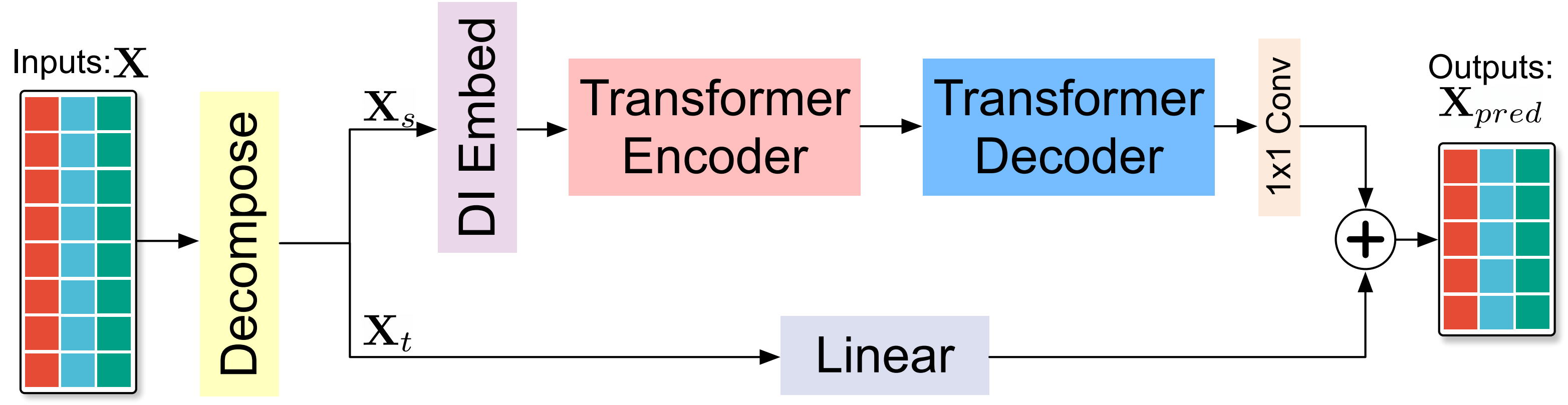
For each ablation experiment, the full encoder–decoder architecture serves as our baseline. We illustrate this design using the Dozerformer model in Figure [fig:encoder-decoder], which provides a representative example of the encoder–decoder structure employed across Transformer-based forecasting models.
The input consists of a historical multivariate time series \(X \in \mathbb{R}^{I \times D}\), where \(D\) denotes the number of variables observed over \(I\) past time steps. The forecasting objective is to predict the next \(O\) future steps, denoted as \(\hat{Y} \in \mathbb{R}^{O \times D}\).
In Dozerformer, a decomposition operator first separates the raw time series into seasonal and trend components, denoted by \(X_s\) and \(X_t\), respectively. The seasonal component \(X_s\) is embedded into a latent space of dimension \(d_{\text{model}}\) and is provided as input to both the Transformer encoder and the Transformer decoder. The encoder is designed to capture long-range temporal dependencies over the full historical window, which is typically set to a large context length (e.g., 720 time steps). The input to the Transformer decoder consists of a shorter segment of recent historical values together with placeholders corresponding to the forecasting horizon, where the historical window is typically much shorter (e.g., 96 time steps). A subsequent \(1 \times 1\) convolutional layer reduces the channel dimension to match the original multivariate time series format.
The trend component \(X_t\) is passed directly through a linear projection to generate trend forecasts for the desired horizons. The final prediction is obtained by combining the seasonal and trend components through elementwise summation. This design follows the standard Transformer encoder–decoder paradigm originally introduced for natural language processing and widely adopted in time series forecasting models.
The attention mechanism plays a central role, accounting for the majority of the computational cost and enabling the model to learn temporal dependencies from the input sequence. The self-attention module projects the embedded input sequence \(E\) into queries \(Q = E W_Q\), keys \(K = E W_K\), and values \(V = E W_V\) using learned linear transformations. The attention output is computed as \[\mathrm{Attention}(Q,K,V)=\mathrm{Softmax}\!\left(\frac{QK^T}{\sqrt{d_k}}\right)V,\] where \(W_Q\), \(W_K\), and \(W_V\) are projection matrices and \(d_k\) denotes the key dimension. To improve efficiency while preserving long-range temporal modeling, Dozerformer employs a sparse attention mechanism that combines local and stride-based patterns, reducing the quadratic cost of standard self-attention while maintaining the ability to capture both short- and long-term dependencies.
3.2 Encoder-Only Architecture
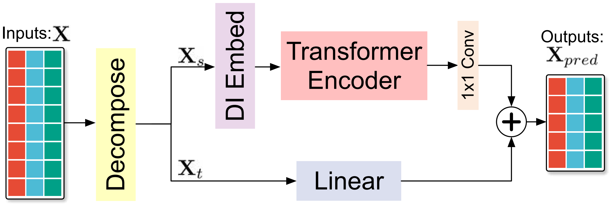
Figure 1 illustrates the encoder-only variant, shown here using Dozerformer as a representative architecture. In this configuration, the decoder is removed and forecasts are generated directly from the encoder’s final hidden states. After the historical input sequence is processed through stacked Dozerformer encoder blocks, the resulting contextual representations are passed through a linear projection layer to produce predictions. This design eliminates the autoregressive decoding stage, thereby reducing model complexity and inference time, while relying solely on the encoder’s ability to capture temporal dependencies over the full input sequence.
3.3 Decoder-Only Architecture
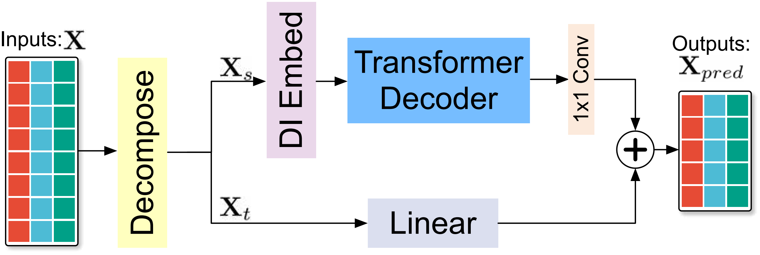
Figure 2 illustrates the decoder-only variant, again using Dozerformer as a representative example. In this configuration, the encoder is removed and the model relies exclusively on an autoregressive decoder. The historical input sequence is embedded and passed directly to the decoder, which predicts future time steps sequentially. At each step, the model attends to previously generated outputs through masked self-attention and applies the sparse Dozer attention pattern to improve efficiency. This design substantially simplifies the overall architecture by removing the encoder while preserving the decoder’s ability to model both short- and long-term temporal dependencies.
3.4 Architectural Specifications
We examine three architectural variants to assess the respective contributions of the encoder and decoder in Transformer-based multivariate time series forecasting. The primary analysis is conducted using the Dozerformer framework, which serves as our main experimental backbone. For Dozerformer, the first variant is the standard encoder–decoder model, which follows the original design and serves as the baseline. The second variant removes the decoder and generates predictions directly from the encoder’s contextual representations. The third variant removes the encoder and relies solely on the decoder’s autoregressive dynamics.
The same ablation protocol is then applied to four additional Transformer-based forecasting models, vanilla Transformer, Informer, FEDformer, and Autoformer, by removing either the encoder or the decoder while preserving each model’s original architectural components. Within each model family, all variants share the same embedding layers, positional encodings, normalization schemes, residual connections, and model-specific attention mechanisms. Aside from the removal of the encoder or decoder, all architectural hyperparameters, including hidden dimension, number of layers, feed-forward size, activation function, and dropout, are kept identical to ensure a fair comparison. This controlled setup isolates the influence of each architectural component while minimizing confounding effects from auxiliary design choices.
3.5 Accuracy Results Across Architectures
We present detailed ablation results for Dozerformer, which serves as the primary experimental backbone of our study. To evaluate whether the observed encoder–decoder behavior generalizes beyond a single architecture, we also have reported corresponding results for four additional Transformer-based forecasting models: Informer, vanilla Transformer, FEDformer, and Autoformer. For each model, we compare the full encoder–decoder configuration with encoder-only and decoder-only variants under identical experimental settings.
| Dataset | H | Dozerformer | Encoder-only | Decoder-only | |||
| MSE | MAE | MSE | MAE | MSE | MAE | ||
| ETTh1 | 96 | 0.364 | 0.385 | 0.357 | 0.397 | 0.367 | 0.391 |
| 192 | 0.404 | 0.410 | 0.416 | 0.420 | 0.407 | 0.416 | |
| 336 | 0.431 | 0.432 | 0.445 | 0.433 | 0.427 | 0.430 | |
| 720 | 0.453 | 0.463 | 0.443 | 0.458 | 0.446 | 0.458 | |
| ETTh2 | 96 | 0.278 | 0.335 | 0.274 | 0.331 | 0.274 | 0.331 |
| 192 | 0.340 | 0.376 | 0.342 | 0.376 | 0.341 | 0.375 | |
| 336 | 0.365 | 0.403 | 0.366 | 0.401 | 0.366 | 0.401 | |
| 720 | 0.400 | 0.435 | 0.381 | 0.421 | 0.399 | 0.435 | |
| ETTm1 | 96 | 0.291 | 0.332 | 0.287 | 0.332 | 0.291 | 0.337 |
| 192 | 0.332 | 0.355 | 0.333 | 0.358 | 0.327 | 0.358 | |
| 336 | 0.367 | 0.376 | 0.358 | 0.374 | 0.361 | 0.379 | |
| 720 | 0.425 | 0.410 | 0.413 | 0.407 | 0.412 | 0.408 | |
| ETTm2 | 96 | 0.164 | 0.248 | 0.159 | 0.243 | 0.161 | 0.248 |
| 192 | 0.223 | 0.291 | 0.214 | 0.284 | 0.218 | 0.286 | |
| 336 | 0.273 | 0.325 | 0.269 | 0.322 | 0.272 | 0.323 | |
| 720 | 0.356 | 0.380 | 0.357 | 0.379 | 0.355 | 0.378 | |
| Weather | 96 | 0.146 | 0.189 | 0.148 | 0.191 | 0.154 | 0.199 |
| 192 | 0.188 | 0.230 | 0.196 | 0.236 | 0.195 | 0.238 | |
| 336 | 0.238 | 0.271 | 0.251 | 0.278 | 0.249 | 0.280 | |
| 720 | 0.310 | 0.322 | 0.319 | 0.329 | 0.316 | 0.330 | |
| ILI | 24 | 1.602 | 0.837 | 1.801 | 0.843 | 1.786 | 0.824 |
| 36 | 1.371 | 0.761 | 1.845 | 0.851 | 1.815 | 0.845 | |
| 48 | 1.371 | 0.822 | 2.098 | 0.934 | 2.039 | 0.907 | |
| 60 | 1.696 | 0.884 | 1.995 | 0.938 | 2.033 | 0.950 | |
| Dataset | H | Informer | Encoder-only | Decoder-only | |||
| MSE | MAE | MSE | MAE | MSE | MAE | ||
| ETTh1 | 96 | 1.416 | 0.976 | 1.663 | 1.028 | 0.937 | 0.739 |
| 192 | 1.643 | 1.025 | 1.681 | 1.009 | 0.965 | 0.741 | |
| 336 | 1.652 | 0.965 | 1.582 | 0.948 | 1.094 | 0.820 | |
| 720 | 1.497 | 0.962 | 1.546 | 0.979 | 1.183 | 0.856 | |
| ETTh2 | 96 | 7.362 | 2.227 | 9.927 | 2.795 | 3.587 | 1.550 |
| 192 | 6.568 | 2.028 | 6.368 | 2.201 | 5.695 | 2.040 | |
| 336 | 6.123 | 2.063 | 4.662 | 1.880 | 4.297 | 1.738 | |
| 720 | 5.324 | 1.973 | 3.613 | 1.666 | 3.881 | 1.723 | |
| ETTm1 | 96 | 1.063 | 0.786 | 0.688 | 0.627 | 0.871 | 0.670 |
| 192 | 1.730 | 1.002 | 0.968 | 0.775 | 0.969 | 0.724 | |
| 336 | 1.356 | 0.905 | 1.037 | 0.813 | 1.021 | 0.773 | |
| 720 | 1.406 | 0.926 | 1.303 | 0.901 | 1.026 | 0.779 | |
| ETTm2 | 96 | 1.046 | 0.789 | 2.499 | 1.301 | 0.459 | 0.502 |
| 192 | 2.278 | 1.193 | 3.305 | 1.562 | 0.959 | 0.774 | |
| 336 | 3.015 | 1.372 | 4.213 | 1.725 | 1.615 | 1.003 | |
| 720 | 8.390 | 2.330 | 8.184 | 2.593 | 2.380 | 1.175 | |
| Dataset | H | Transformer | Encoder-only | Decoder-only | |||
| MSE | MAE | MSE | MAE | MSE | MAE | ||
| ETTh1 | 96 | 1.791 | 1.128 | 1.427 | 1.013 | 0.877 | 0.715 |
| 192 | 2.053 | 1.237 | 1.852 | 1.166 | 0.894 | 0.735 | |
| 336 | 1.692 | 1.063 | 1.639 | 1.058 | 1.053 | 0.829 | |
| 720 | 1.299 | 0.942 | 1.570 | 1.060 | 1.083 | 0.852 | |
| ETTh2 | 96 | 2.263 | 1.303 | 3.417 | 1.497 | 1.921 | 1.147 |
| 192 | 5.945 | 2.002 | 5.019 | 1.945 | 3.852 | 1.615 | |
| 336 | 6.092 | 2.110 | 3.854 | 1.686 | 5.395 | 1.955 | |
| 720 | 4.437 | 1.773 | 4.856 | 1.848 | 5.037 | 1.927 | |
| ETTm1 | 96 | 0.597 | 0.553 | 0.600 | 0.581 | 0.503 | 0.505 |
| 192 | 0.740 | 0.643 | 0.725 | 0.634 | 0.643 | 0.606 | |
| 336 | 0.857 | 0.736 | 1.166 | 0.852 | 0.871 | 0.726 | |
| 720 | 1.018 | 0.796 | 1.115 | 0.802 | 0.786 | 0.675 | |
| ETTm2 | 96 | 1.084 | 0.798 | 1.936 | 1.060 | 0.321 | 0.410 |
| 192 | 1.812 | 1.068 | 2.549 | 1.287 | 0.894 | 0.706 | |
| 336 | 2.968 | 1.442 | 3.777 | 1.619 | 1.035 | 0.802 | |
| 720 | 8.180 | 2.369 | 7.241 | 2.351 | 2.589 | 1.258 | |
| Dataset | H | FEDformer | Encoder-only | Decoder-only | |||
| MSE | MAE | MSE | MAE | MSE | MAE | ||
| ETTh1 | 96 | 0.448 | 0.482 | 0.995 | 0.819 | 0.446 | 0.482 |
| 192 | 0.467 | 0.490 | 0.974 | 0.794 | 0.458 | 0.482 | |
| 336 | 0.513 | 0.519 | 0.912 | 0.737 | 0.484 | 0.501 | |
| 720 | 0.710 | 0.640 | 0.855 | 0.718 | 0.579 | 0.563 | |
| ETTh2 | 96 | 0.403 | 0.449 | 3.200 | 1.401 | 0.409 | 0.457 |
| 192 | 0.420 | 0.462 | 3.266 | 1.405 | 0.416 | 0.461 | |
| 336 | 0.438 | 0.472 | 3.035 | 1.326 | 0.431 | 0.469 | |
| 720 | 0.438 | 0.488 | 3.061 | 1.331 | 0.493 | 0.512 | |
| ETTm1 | 96 | 0.365 | 0.429 | 1.113 | 0.851 | 0.360 | 0.423 |
| 192 | 0.388 | 0.437 | 1.090 | 0.841 | 0.374 | 0.425 | |
| 336 | 0.383 | 0.428 | 1.102 | 0.828 | 0.385 | 0.430 | |
| 720 | 0.443 | 0.462 | 0.992 | 0.762 | 0.438 | 0.458 | |
| ETTm2 | 96 | 0.301 | 0.363 | 2.915 | 1.355 | 0.302 | 0.365 |
| 192 | 0.332 | 0.383 | 3.308 | 1.445 | 0.331 | 0.382 | |
| 336 | 0.361 | 0.397 | 3.483 | 1.457 | 0.359 | 0.396 | |
| 720 | 0.434 | 0.449 | 3.292 | 1.384 | 0.427 | 0.446 | |
| Dataset | H | Autoformer | Encoder-only | Decoder-only | |||
| MSE | MAE | MSE | MAE | MSE | MAE | ||
| ETTh1 | 96 | 0.493 | 0.506 | 0.852 | 0.724 | 0.511 | 0.510 |
| 192 | 0.529 | 0.537 | 0.848 | 0.715 | 0.501 | 0.510 | |
| 336 | 0.649 | 0.614 | 0.867 | 0.730 | 0.528 | 0.528 | |
| 720 | 0.732 | 0.666 | 0.870 | 0.724 | 0.584 | 0.576 | |
| ETTh2 | 96 | 0.446 | 0.487 | 3.127 | 1.351 | 0.406 | 0.458 |
| 192 | 0.755 | 0.669 | 3.105 | 1.340 | 0.434 | 0.477 | |
| 336 | 0.550 | 0.567 | 3.061 | 1.325 | 0.431 | 0.475 | |
| 720 | 1.151 | 0.860 | 3.093 | 1.335 | 0.502 | 0.512 | |
| ETTm1 | 96 | 0.541 | 0.504 | 1.010 | 0.764 | 0.391 | 0.435 |
| 192 | 0.504 | 0.500 | 0.961 | 0.751 | 0.391 | 0.435 | |
| 336 | 0.620 | 0.568 | 0.979 | 0.757 | 0.537 | 0.496 | |
| 720 | 0.562 | 0.525 | 0.995 | 0.757 | 0.569 | 0.511 | |
| ETTm2 | 96 | 0.314 | 0.376 | 3.149 | 1.363 | 0.301 | 0.363 |
| 192 | 0.497 | 0.466 | 3.152 | 1.361 | 0.330 | 0.381 | |
| 336 | 0.415 | 0.458 | 3.143 | 1.360 | 0.362 | 0.399 | |
| 720 | 0.592 | 0.562 | 3.131 | 1.353 | 0.416 | 0.440 | |
3.6 Accuracy Analysis
Table 1 reports the forecasting accuracy of the three Dozerformer variants: the full encoder–decoder, the encoder-only, and the decoder-only configurations. Evaluations are conducted on six multivariate time series datasets under four prediction horizons each, yielding a total of twenty-four forecasting tasks. For each task, we report both mean squared error (MSE) and mean absolute error (MAE).
Across these tasks, the decoder-only variant achieves lower or equal MSE compared with the full encoder–decoder configuration in twelve out of twenty-four settings and lower or equal MAE in twelve settings as well. When both metrics are considered jointly, the decoder-only model is competitive in fifteen out of twenty-four forecasting tasks. These results indicate that removing the encoder does not systematically degrade forecasting accuracy and that, in many settings, the decoder alone is sufficient to capture the dominant temporal dependencies present in multivariate time series data.
Dataset-level trends provide further insight into when encoder removal is most effective. On ETTm1 and ETTm2, which exhibit relatively regular and periodic temporal structure, the decoder-only variant frequently matches or surpasses the full encoder–decoder across nearly all horizons, including long-range forecasts of 720 steps. This behavior suggests that when temporal dynamics are stable and repetitive, autoregressive decoding with masked self-attention is capable of modeling both short- and long-term dependencies without relying on additional encoder representations.
In contrast, on ETTh1 and ETTh2, which contain more irregular dynamics and higher noise levels, the decoder-only variant remains competitive at longer horizons, particularly 336 and 720 steps, but is outperformed by the full encoder–decoder configuration at shorter horizons in some cases. This pattern indicates that encoder representations can become beneficial when long-range dependencies are more difficult to infer directly from recent history or when noise obscures salient temporal structure.
On the Weather dataset, which combines strong seasonal components with highly variable short-term fluctuations, the full encoder–decoder model achieves the best overall performance across most horizons. A similar trend is observed on the ILI dataset, which involves sparse, low-frequency observations and long seasonal cycles. In these settings, retaining the encoder appears to improve stability and generalization, particularly for longer forecasting horizons where limited historical signal must be extrapolated over extended time spans.
The encoder-only variant exhibits limited and inconsistent benefits. While it achieves performance comparable to or slightly better than the full model in a small number of structured settings, such as ETTm1 at short horizons, it degrades substantially on more complex datasets such as Weather and ILI. This suggests that the encoder alone is often insufficient for accurate forecasting, particularly when autoregressive dynamics play a central role in modeling temporal evolution.
To assess whether these findings generalize beyond Dozerformer, we report corresponding ablation results for four additional Transformer-based forecasting architectures, vanilla Transformer, Informer, FEDformer, and Autoformer, in Tables 2–5. Across these models, the decoder-only configuration consistently achieves the strongest or near-strongest performance in the majority of forecasting tasks. Notably, the performance gains observed for decoder-only variants are often substantially larger than those observed in Dozerformer, particularly for the vanilla Transformer and Informer architectures.
For the vanilla Transformer, removing the encoder leads to dramatic improvements across nearly all datasets and horizons, with error reductions that are often several times larger than those achieved by the full encoder–decoder model. Similar behavior is observed for Informer, where the decoder-only variant frequently outperforms both the full model and the encoder-only variant by a wide margin. These results indicate that, in architectures with weaker or more generic inductive biases, the encoder may introduce redundancy or noise rather than complementary information.
In contrast, models with stronger time-series-specific inductive biases, such as Dozerformer, FEDformer, and Autoformer, exhibit a more nuanced trade-off. While decoder-only variants remain highly competitive and often superior, the encoder sees partial utility on more challenging datasets, particularly those characterized by irregular sampling, long seasonal cycles, or complex trend–seasonality interactions. This suggests that the effectiveness of encoder removal is architecture- and data-dependent, rather than universally optimal.
Overall, these results demonstrate that encoder–decoder redundancy is not an isolated phenomenon tied to a single model, but a recurring pattern across diverse Transformer-based forecasting architectures. In many practical forecasting settings, especially those involving regular or moderately structured temporal dynamics, the decoder emerges as the primary contributor to predictive performance, while the encoder provides limited or conditional benefits. These findings motivate a reevaluation of encoder–decoder symmetry in time series forecasting and highlight decoder-centric designs as a promising direction for building simpler, more efficient, and often more accurate forecasting models.
[top]
4 Conclusion
This work reexamines the architectural assumptions underlying Transformer-based time series forecasting, particularly the necessity of the encoder–decoder structure inherited from natural language processing. Using Dozerformer as a representative backbone, we conducted a systematic ablation study comparing three configurations, encoder–decoder, encoder-only, and decoder-only, across six benchmark datasets and multiple forecasting horizons. To assess generality, the same ablation protocol was applied to four additional Transformer-based forecasting models: vanilla Transformer, Informer, FEDformer, and Autoformer.
Our results show that decoder-only designs often provide the most favorable balance between forecasting accuracy and architectural simplicity. In the Dozerformer setting, the decoder-only variant matches or outperforms the full encoder–decoder model in fifteen of twenty-four forecasting tasks, with particularly strong performance on structured datasets such as ETTm1 and ETTm2. Across additional architectures, similar accuracy trends are observed, most notably for the vanilla Transformer, though the relative benefit of retaining the encoder varies by dataset and model family.
Overall, these findings challenge the assumption that encoder–decoder symmetry is universally necessary for time series forecasting. The decoder frequently emerges as the primary component responsible for modeling temporal dependencies, while the encoder provides uneven benefits that depend on data complexity and temporal structure. This suggests that decoder-centric architectures, when carefully designed, offer a promising direction for building simpler, more efficient, and better-aligned Transformer models for time series forecasting.
Acknowledments This research was conducted at
Missouri State University with support from the Department of
Mathematics and the Department of Computer Science.
Last modified September 13, 2026.
Math rendered with MathJax. Embedded diagrams are rendered from the manuscript source itself.
Best viewed with a browser that still believes HTML tables are a layout system.